How to get your robots to carry out their autonomous motion in real life
Recently I was part of a team whose task was to figure out the motion planning for a Copernicus Robot such that it can avoid obstacles and reach the goal autonomously. But before we dive into how I achieved that let's get a few basics right.
Few ideas work on the first try. Iteration is key to innovation.
- Sebastian Thrun
What is motion planning?
Motion planning is a term used in robotics for the process of breaking down the desired movement task into discrete motions that satisfy movement constraints and possibly optimize some aspect of the movement.
What are the usual approaches for it?
Collision avoidance algorithm is mainly of 2 types: global and local. Some of the global techniques are graph-based, potential field methods and cell decomposition. You can check out the article I wrote about a graph-based approach for a multirobot system here. Global approaches require a complete model of the robot and environment to plan the path. This makes them a bit slow to avoid fast moving obstacles and also if the environment model is not completely accurate.
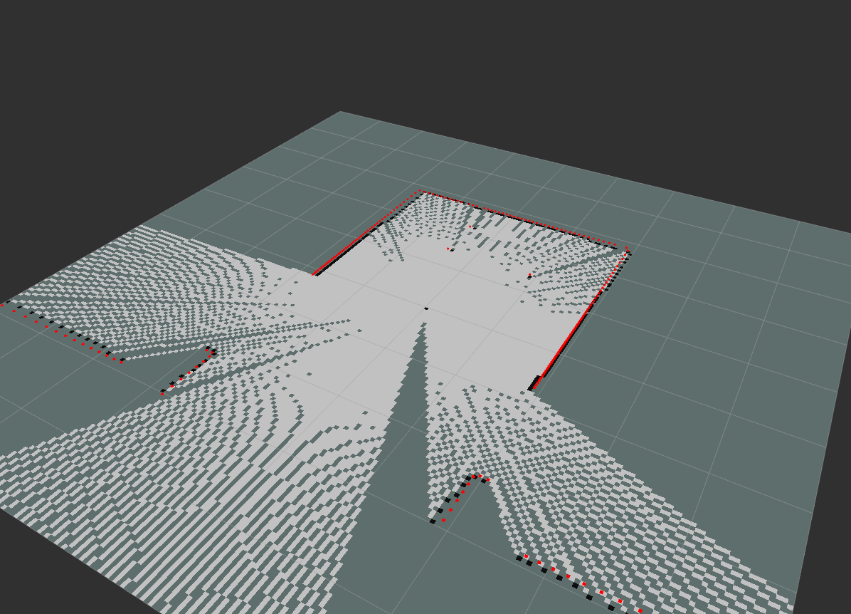
Whereas local planner considers only a small part of the entire model to make the decisions. But they usually provide a solution that is less optimal and it is more prone to being stuck in local-minima. But they can make a decision at a faster pace and are able to make decisions in a partially available world model. Vector field histogram is a type of local planner approach which uses an occupancy grid to form a model of the nearby environment using sensors. Utilizing the occupancy grid and Artificial Potential Field (APF) it plans the path for the robot.
Shortcomings of previous approaches and Dynamic Window Approach (DWA)?
All the approaches discussed above don't really take the limitations of the robot into consideration (like max acceleration). To deal with this DWA was proposed.
With the introduction out the way let's get to how DWA works!

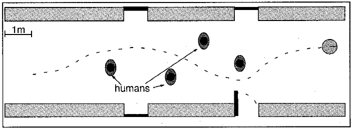
The scope of the article will mainly deal with the algorithm proposed in the original paper[1].
Equations defining robot drive
To be able to provide with motion plan within the limitation of the robot we need to model the robot's drive (How does the robot move). To simplify things we'll consider it to be a mobile robot with a differential drive
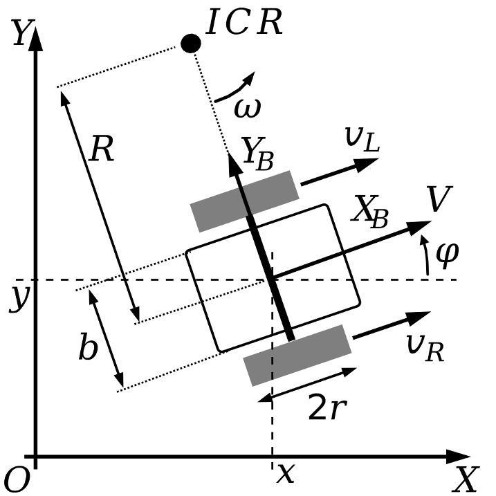
General motion equations can be written as: $$ x(t_{n}) = x(t_{0}) + \int_{t_{0}}^{t_{n}}v(t) \cdot \cos(\theta(t)) dt \\[2em] y(t_{n}) = y(t_{0}) + \int_{t_{0}}^{t_{n}}v(t) \cdot \sin(\theta(t)) dt $$ where, $$ x(t_{n})\space and\space y(t_{n})\space is\space the\space position\space of\space the\space robot\space at\space time\space t_{n}\\ and\space v(t) \space denotes \space velocity \space at \space time \space t\\ and\space \theta(t) denotes \space orientation \space at \space time \space t $$ Rewriting v(t) and θ(t) in terms of initial configuration and acceleration as: $$ x(t_{n}) = x(t_{0}) + \int_{t_{0}}^{t_{n}} \bigg( v(t_0) + \int_{t_0}^t a(\hat{t}) d\hat{t}\bigg) \cdot \cos\bigg(\theta(t_0) + \int_{t_0}^t \Big( \omega(t_0) + \int_{t_0}^t \alpha(\hat{t}) d\hat{t} \Big) dt\bigg)\\[2em] y(t_{n}) = y(t_{0}) + \int_{t_{0}}^{t_{n}} \bigg( v(t_0) + \int_{t_0}^t a(\hat{t}) d\hat{t}\bigg) \cdot \sin\bigg(\theta(t_0) + \int_{t_0}^t \Big( \omega(t_0) + \int_{t_0}^t \alpha(\hat{t}) d\hat{t} \Big) dt\bigg) $$ where, $$ a(\hat{t})\space and\space \alpha(\hat{t})\space are\space linear\space acceleration\\ and\space angular\space acceleration\\ in\space time\space interval\space \hat{t}\in[t_0,t] $$ With this, we have equations that are based on initial configuration and acceleration only!
Considering hardware restriction, all the variable values will be discrete in nature and hence the above equations need to be discretized. Further, we can simplify them by approximating constant robot velocity for a short interval of time [ti,ti+1]. Doing so introduces error in the trajectory but because the robot's position is measured periodically we can neglect it. The final motion equation can be written as, $$ x(t_{n}) = x(t_{0}) + \sum_{i=0}^{n-1}\int_{t_{i}}^{t_{i+1}}v_i \cdot \cos\bigg(\theta(t_i) + \omega_i \cdot (\hat{t}-t_i)\bigg)d\hat{t}\\[2em] y(t_{n}) = y(t_{0}) + \sum_{i=0}^{n-1}\int_{t_{i}}^{t_{i+1}}v_i \cdot \sin\bigg(\theta(t_i) + \omega_i \cdot (\hat{t}-t_i)\bigg)d\hat{t} $$ where, $$ n\space denotes \space number \space of \space time \space intervals $$
After further simplification of the integral one can transform the above equations into a circular trajectory equation. Something like this, $$ (F^i_x - M^i_x)^2 + (F^i_y - M^i_y)^2 = (\frac{v_i}{\omega_i})^2 $$ where, $$ (M^i_x,M^i_y) \space represents \space center \space of \space i^{th} \space circle $$
DWA Approach
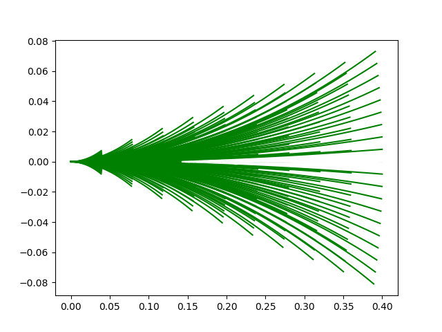
In this approach, the search for the best trajectory is done in the velocity space. The trajectory of the robot is a sequence of circular arcs. Each arc/curvature is defined by (vi,ωi). Hence from the above equations, we can say that to reach the goal point for the next n interval we need to determine (vi,ωi) for each of those n intervals.
Windowing
The way we introduce the dynamics of the robot is by limiting the velocity space being used to find the best trajectory. This operation is called windowing and it restricts the velocities to only the velocities which can be reached within a short interval of time given the max acceleration of the robot.
$$ V_d = \bigg\lbrace(v,\omega) | v\in[v_a - a\cdot t,v_a+a\cdot t] \land \omega \in [\omega_a - \alpha \cdot t, \omega_a + \alpha \cdot t]\bigg\rbrace $$ where, $$ a \space and \space \alpha \space are \space acceleration $$
Avoiding Obstacles
The above space is then again pruned by considering the only safe trajectories. A trajectory is considered safe only when the pair (v,ω) can stop before it reaches the nearest obstacle. $$ V_a = \bigg\lbrace(v,\omega) | v\le\sqrt{2\cdot dist(v,\omega)\cdot\dot{v_b}} \land \omega\le\sqrt{2\cdot dist(v,\omega)\cdot\dot{\omega_b}}\bigg\rbrace $$
Finally we can write the resulting search space as $$ V_r = V_s \cap V_a \cap V_d $$
Optimization of the trajectory
Next, we need to select the best trajectory amongst the admissible ones. To do this we use the following optimization function in the Vr space.
$$
G(v,\omega) = \sigma(\alpha\cdot heading(v,\omega) + \beta \cdot dist(v,\omega) + \gamma \cdot velocity(v,\omega))
$$
where,
$$
\sigma \space is \space for \space smoothing
$$
Amongst a set of given trajectory the one with highest G(v,ω) is selected.
Target Heading
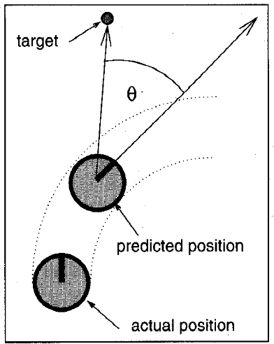
heading(x,ω) function evaluates the alignment of the robot to the target heading. It is given by 180-θ, where θ is the delta between the heading of the robot after it undertakes a given trajectory and the angle goal point makes from the current position of the robot.
Clearance
dist(x,ω) function evaluates the minimum distance to the nearest obstacle when a given trajectory is followed. This helps to select the trajectory having the highest clearance from the obstacles.
Velocity
velocity(x,ω) function just returns the translation velocity robot will have at the end of the trajectory. This helps to select the trajectory which goes the fastest.
Distance to Goal
goalDistance(x,ω) function returns the distance between the robot and the goal after it undertakes the given trajectory. This is an addition to the parameters given in the paper. This helps to undertake a trajectory that brings the robot closest to the goal. This is extremely helpful when one allows negative velocities in the window.
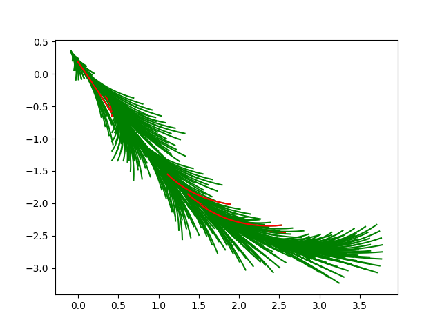
Results
The algorithm was implemented in C++ and ROS was used as middleware between the program and the robot. The following were the weights and parameters of the robot.
PREDICT_TIME: 2.0 # time interval size
HZ: 10 #1/deltaT
HEADING_COST_GAIN: 0.5 # Difference in heading between the traj final orientation and goal orientation at present
OBSTACLE_COST_GAIN: 1.0 # Applied on the distance to the nearest obstacle
SPEED_COST_GAIN: 0.2 # Cost factor for the speed, used to maximize the speed of the robot
TO_GOAL_COST_GAIN: 0.8 # Cost factor on how far robot is wrt goal position

MAX_VELOCITY: 0.5  #Max vel of robot
MIN_VELOCITY: 0.0 #Min vel of robot
MAX_ACCELERATION: 1.0 #Max acc of robot
MAX_YAWRATE: 0.8 #Max angular vel of robot
MAX_D_YAWRATE: 2.0 #Max angular acceleration of robot
Implementation Result
Video of simulation and implementation on a real robot can be seen here:
Observations
As we discussed in the usual approaches local planning gets stuck in local minima and hence needs some additional force (recovery behavior)to get out of it. In the given implementation this part was lacking and hence to mimick recovery behavior the robot was rotated by hand so that it could come out of the given minima. Another realization that happened while making the program was that DWA requires a fast loop time and hence algorithms implemented on python aren't best suited for this purpose.
Up-Next
The code base is available here. In coming days will upload a documentation of what each function does, so stay tuned!
Also fun-fact you can subscribe to the blog using RSS! For Firefox users you can use Livemark for this.
$ press CTRL+W to end the session.
[1] D. Fox, W. Burgard, and S.Thrun, "The dynamic window approach to collision avoidance", IEEE Robotics Automation Magazine, 1997.